Today we’re talking about the Naive Bayes Classifier. Not to be confused with the everything else that has Bayes’ name on it.  There’s a whole branch of Bayesian statistics. It’s all very interesting, but today we’re just talking about the parts it takes to build the most basic of classifiers, why it’s done the way it is and when it’s likely to work.

Building the Classifier

The Naive Bayes classifier is a generative model (as opposed to a discriminative model), which means it works by building an approximate statistical model, and then using that model to calculate probabilities which are then used to make predictions. What makes the Naive Bayes model so naive is that all the inputs are assumed to be independent of each other (i.e. knowing one input doesn’t give you any information about any of the others), and typically the distributions are assumed to be a fixed shape.  With these assumptions the “training” portion of the algorithm just consists of calculating the means and standard deviations for each input separately for each class.

For the sake of brevity I’m going to assume you can figure out how to calculate variances. If not there’s a nice Wikipedia article devoted to it. The important part here is that you calculate a separate distribution for each class, so that we can compare their likelihoods on new inputs. For my example I use the binary version of the algorithm, but there’s nothing stopping you from making a version that works on an arbitrary number of classes.

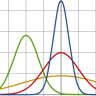
Alright, so we’ve determined the means and variances, but we still have to decide what type of distribution to use before we can calculate any probabilities.  We could use our data to determine what type of distributions to use, or we could just pick a winner and hope for the best.  Let’s go with the normal distribution. This algorithm is called naive after all, and I’m feeling lucky.

 

Why the normal distribution you say? Normal distributions tend to pop up frequently in “natural” data. To understand this we need look no further than the central limit theorem, which states “given certain conditions, the arithmetic mean of a sufficiently large number of iterates of independent random variables, each with a well-defined expected value and well-defined variance, will be approximately normally distributed”. That is, if the thing you’re interested in is actually the result of adding a whole bunch of smaller random things together, no matter what their distributions are, then it’ll be close to a normal distribution.

Applying the Classifier

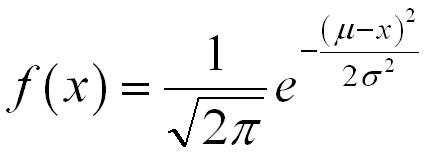
Assuming a normal distribution all we have to do is plug our new x’s into the above formula with our mean (µ) and our variance ( σ^2 is variance since σ is standard deviation in that formula).  Since each of our variables is assumed to be independent from the others the probability of seeing the entire x vector is the multiple of seeing each piece.

That’s all well and good, but we’re not interested in the probability of seeing this X. We’re interested in the probability of this X being in each class.  We can get the probability we actually want by applying Bayes’ Theorem:

 

In this case A is the probability of being positive, and B is the probability of this input vector. Thus the probability of being positive given this input vector ( what we want) is the probability of this input vector given that we’re positive (P( B|A) = what we calculated above) times the probability of being positive overall divided by the probability of this input vector overall.  We can get the probability of being positive overall by counting up what fraction of the total training data was positive, but what about the overall probability of the input data point? We didn’t calculate that.

Here’s the trick: we’re going to assume all data points are either positive or negative cases. That is P(positive) + P(negative) = 1.  Given that assumption we only have to care about the relative probability of positive versus negative. When we get to the end we can just divide out by the sum to get the absolute probabilities. Since P(B) above is the same for both positive and negative cases it doesn’t effect the final result and we can safely ignore it. Likewise, that 1/sqrt(2*pi) term on the normal is the same for both and has no effect on the final result.  All we really need to do is calculate the chance of the input being in each class and then multiply that by the overall chance of that class.

One final trick before I get to the final code: move the exponential outside of the loop. The multiple of a bunch of exponentials  is the exponential of a sum: e^a * e^b = e^(a+b).  It’s not a big deal, but it saves a few unnecessary computations.

Conclusion

This function and the constructor at the top are all you need to make a Naive Bayes Classifier. Congratulations, you can now predictively model things! Unfortunately, this is one of the simpler, and generally weaker algorithms. That being said, it’s a lot better than nothing, and sometimes it’s “good enough”. Let’s talk about when that is.

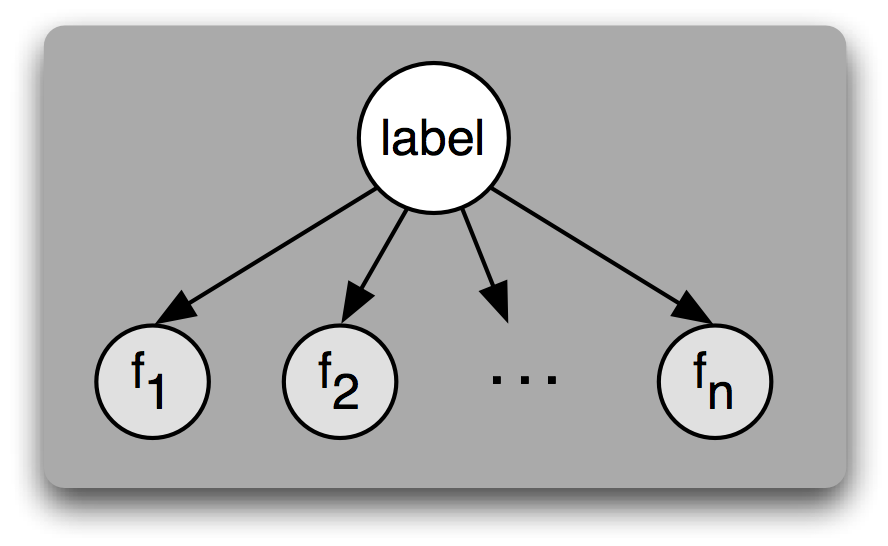
This is a picture of a Naive Bayesian network. I’m not covering Bayesian networks in this article, but what’s important is that each arrow in a Bayesian network represents a dependence. In a Naive Bayesian network each input is treated as being dependent on only the output class or label. This and the assumption of normal distributions make up the inductive bias of the Naive Bayes classifier.

If your inputs are dependent on the class but not dependent on each other and those inputs are random variables that could be made by adding up lots of other little random variables then this Naive Bayes Classifier will work pretty well. Naive Bayes also has one other significant advantage: missing data. Since all the variables are considered independently, removing one from the probability calculation produces the same result as if you had trained without that variable to begin with; It’s pretty straightforward to build a Naive Bayes classifier that handles data with lots of null values.  Of course, the primary reason these get used as much as they do is because they’re easy to understand and quick to program and train. Training, if you can call it that, can be done in a single loop over the data, which is to say this is one of the fastest “machine learning” algorithms in existence.

The reason not to use a Naive Bayes classifier? Accuracy.  More sophisticated techniques can get much higher accuracy and deal with much more complex problems. I will be getting into all of the fancier techniques I can find as well as delving a bit more into general topics such as optimization, numerical and data structure tricks, and testing (so you don’t have to take my word on the accuracy).