 Decision trees make predictions by asking a series of simple questions. I’ll show you how to train one using a greedy approach, how to build decision forests to take advantage of the wisdom of crowds, and then we’ll be optimizing a rotation forest to build a fast version of one of the most accurate classifiers available.
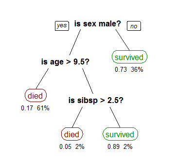
We’re back on classification problems today, but this time we’re dialing down the statistics in favor of a more data structures driven approach. We’re going to build trees that recursively cut up our input space in an effort to separate our classes. The simplest form of a decision tree looks like a flow chart of binary questions. Each branch asks if a single variable is greater than or less than a certain value, and each leaf outputs a probability. Predicting a class for a new input is as simple as walking down the tree, and then outputting the class with the highest probability when you reach a leaf.
I expect this article to be a bit on the long side, so I’m going to make a few simplifying assumptions to get things rolling. Today we’re only looking at fixed length numerical feature vectors for binary classification. That is, every input vector is a set size and isn’t missing any values, and all the inputs are numbers as opposed to categorical, string, or other data. We’re also only looking at positive vs negative classification. This is the classic easy variety of a binary classification problem. For all intents and purposes it’s a solved problem, and this article is about one of the better solutions.
Alright, so using a tree once it’s built is easy, now how do we actually build one? It turns out building the “best” tree is an NP-complete problem. It would take a very long time, and we don’t really need the best tree anyway. Actually, since we’ll ultimately be building multiple trees and don’t want them all to be the same, we don’t even want the “best” tree. What we need is an algorithm that produces a lot of different pretty good trees quickly.
That algorithm is a heuristic greedy algorithm. Using some sort of rule of thumb for how good a tree is you make every decision like it’ll be your last . Given my data-set, what’s the best single question I could ask that would tell me as much as possible about what the class is of any data point? Split the data on that question, and then apply the same technique to each of the two children. Using this approach we avoid the combinatorial explosion that results from trying to find multiple splits that together form the best tree, and we still get pretty good trees as long as we pick a good heuristic.
Asking the Right Question
What does it mean to pick a question that “tells as much as possible about what the class is”? For this we can make use of the concept of Shannon entropy from information theory. Entropy in information theory is a measure of the average unpredictability in a random variable which happens to be the same thing as its information content. We can use formulas from information theory to approximate the number of bits we would need to store our class information.
![]()
Given the probabilities of each class, multiply each by its log and add them up, and that gives you the negative of the amount of information in each instance. Since, we’re limiting ourselves to binary classification we only have one probability (p): the probability of a positive case, and then the probability of a negative case is one minus that, so you end up with:
 = -1* ( p * log_2 (p) + (1-p)*log_2(1-p) )")
This represents the amount of bits we’d expect to need to store each class value where the chance of a positive instance is p. If we look at the graph of this function what we’ll see is a pretty simple curve that’s zero if we have all one class, and a whole bit if we have a 50-50 distribution. Then the goal when selecting a question to ask is to minimize the amount of information you will still need, which is the same as (and frequently referred to as) maximizing information gain . It makes sense as that will pick splits that have uneven levels of positive and negative cases.
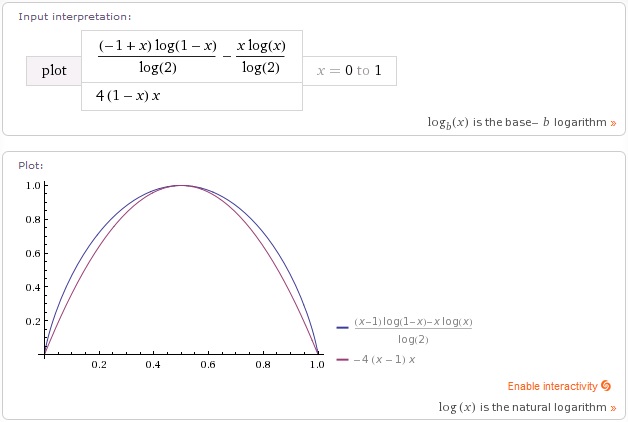 This is by no means the only heuristic you could use. Anything that penalizes balancing positives and negatives at a node, and rewards having mostly one type at a given place will work. As you can see above, a simple parabola 4*x*(1-x) on the probability is almost identical to information gain. This is what I typically use in practice. It’s much cheaper to calculate, and I’ve yet to see any measurable difference in accuracy.
Alright so we have a way to quickly estimate how much info we gain per data point based on the probability of a positive instance, but that doesn’t, by itself, tell us which split is superior. We need to calculate the total amount of information we would gain by making a given split. Any split we make is going to produce two new subsets of training data points. We’re going to have positives and negatives on each side of the split.
Let’s say Lp and Ln for the number of positives and negatives on the left of the split with L=Lp+Ln, and Rp and Rn for the number of positives and negatives on the right side of the split with R=Rp+Rn. Thus the probabilities of positive for each side are Lp/L and Rp/R. We can estimate the information gain from the formula above as 4 * Lp/L * ( 1- Lp/L) . (1-Lp/L) is the same as Ln/L , so that gives us 4 * Lp * Ln/ ( L^2) information per element. This is a relative measure, so we can ignore the constant factor 4, and we want the total information rather than the per element information, so we multiply by the total number of points L in that group. Do the same thing for the right side, and you get:

Building the Decision Tree
There it is: our final score for “how good of a question is this to ask”. Lower is better in this case. Now, that we have this, all we have to do is enumerate every question we could possibly ask, split the data on that question, count up the positives and negatives on each side, and then pick the one with the best score. Luckily, this is not nearly as computationally intensive as it sounds. For one thing we’re only asking questions on a single variable at a time. For another, the score won’t change unless the split plane passes by a data point, so we only need to check once between each pair of neighboring data points, and if we walk through them in order we can just keep track of the positives and negatives as we pass them.
All we really have to do is sort the data points on each variable, and then walk through each sorted list keeping a running total of positives and negatives passed so far which is all we need to calculate the score for that split. Thus the number of possible splits we have to score at each level is only on the order of the #(inputs) * #(training data points). Once we’ve found the best split, only then do we actually have to split the data into two new sets. Actually, the most computationally expensive part of the whole process is sorting the data on each axis. A naive implementation of this algorithm might look something like this:
There are a number of improvements that could be made there. In practice you’ll want to keep splitting recursively until some sort of exit condition is reached, either a maximum depth or a minimum number of points at the node. Something like that, and obviously you’ll want to stop splitting if you reach a node that has all positive or all negative instances.
There’s also a significant performance issue with the above version. Specifically, you end up doing the same sorting work over again every time you recurse. It’s much better to sort the data-points on every axis up front, and then pass those sorted lists down to the children maintaining the sort order as you split. This isn’t terribly complicated, but it does make the code much longer, so I’ve omitted it from the embedded version. If you’re planning to implement just this simple version in the real world I highly recommend checking out the more complicated final version to at least get the presorting optimization.
We can now make a decision tree from our data and use it to make predictions. A decision tree will work great when you have a huge amount of data, but they have a nasty habit of over-fitting if the data has much noise in it. Given enough data, the learning algorithm above could theoretically keep splitting to fit any classification function to an arbitrary level of accuracy. Realistically, we don’t have infinite data, and even if we did, real data tends to be pretty noisy. We usually don’t want to split as much as possible. It’s a good idea to keep 20 or more points in each leaf, so we can drown out outliers and noise, and also so we can get an estimate of probability.
One solution to the over-fitting problem is pruning. Before training we can pull out a tuning set, and set it aside. Then we build the tree on the remaining data as deep as possible. After the tree is built we use the tuning set to see if each branch would actually work better as a leaf. Any branch that gets higher accuracy on the tuning set as a leaf than its sub-tree gets will have its sub-tree pruned and replaced by the leaf. You’ll want to work from the outer most branches toward the root, so any replacement on the outer level will be considered before making replacements on nodes closer to the root.
Random Forests
The other solution, as you may have guessed, is to build decision forests. The general idea is to build a lot of (think 50-ish) trees on random subsets of the data and with slightly different and also random options. Thus you get different trees with more random errors rather than systematic errors. The random errors tend to cancel each other out in aggregate. The results of any one tree may be a bit worse due to the randomness, but averaging the results of all the trees is typically much better in practice than even the best single tree. This phenomenon is semantically similar to the concept of the wisdom of crowds.
The most common variety of decision forest is the Random Forest. It relies on two changes to the way we build our decision trees: random feature selection and bootstrap aggregation. The goal of these changes is to make sure each tree we generate is different. If we generate 50 trees that are all the same then we’re just wasting memory
Bootstrap aggregation is a general meta-algorithm for building ensembles. Which is a fancy way of saying you can train any model(trees in this case) on random sub-samples of your data to make useful groups to help combat over-fitting. Since we typically draw the samples with replacement (allowing the same point to be drawn multiple times) the algorithm itself couldn’t be much simpler.
The other technique employed by random forests is random feature selection. Rather than testing on every feature at every node we randomly select a subset of features to allow splits on. See that “featurefraction” being passed into the tree above? It’s literally as simple as adding if rand.nextDouble()<featurefraction check for splits on this variable otherwise skip checking this variable when looking for the best split. A feature is unlikely to be overlooked at every level of training, so each tree still usually ends up using all relevant variables, but the limitation causes them to be used in a different order, resulting in different but still pretty good trees.
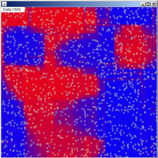
That’s all you need to know to implement a random forest. It’s a pretty solid algorithm for classification problems when a lot of data is available, but it does have a few shortcomings. Since all of the splits are made on a single variable at a time you get this sort of blocky classification function. It sure would be nice if we could fix that while also increasing tree diversity and accuracy.
Rotation Forests
Random feature selection for a random forest just means turning features on and off randomly, but with just a bit more effort we can build random new features. This is essentially what a rotation forest does. Rather than using x and y, one tree might use 2x+3y and 2y-3x for its features to split on. Assuming we use the same features from the root to the leaves (which I highly recommend for efficiency reasons) each individual tree will still be blocky, but their blocks won’t line up. When we average them all together into a forest we’re likely to get something relatively smooth. Additionally, since every split on every tree is still making use of all of the data available (just rotated) the individual trees will tend to have higher accuracies than those in a random forest.
So, how do we generate the new axes, and how do we efficiently use non-axis aligned features in the tree learning process? I’ve seen some literature that suggests using principal component analysis is the best way to generate axes due to the uncorrelated nature of the components [citation needed], but it’s much more complex than I want for this article, and I’ve personally had very good luck just generating axes at random. You do have to be careful though, if your initial features have vastly different ranges/variances a feature with larger numbers can overpower a feature with much smaller numbers.
Normalization
You could scale the input components of your axes by the inverse of the standard deviation to correct for different variances among variables, but I think it’s far more intuitive to just normalize your data upfront. Particularly since normalizing your data is just generally a good idea, and you should probably do it all the time anyway (the polynomials from the last article, yeah, you really need to normalize to get that to run stable on real data).
By “normalizing data” what I mean is shifting and scaling it so that its distribution has means of zero and standard deviations of one. Code for calculating mean and standard deviation is described in the Naive Bayes article, and it’s included in the final code for this article, so I’m not going to talk about that. Once you have the mean and standard deviation in each variable, normalizing the data is simply a matter of subtracting the mean and dividing by the standard deviation for each data point. This should make the majority of your numbers fall in the range of -2 to 2, which puts you in a good position numerically to do things like applying rotations or polynomials, using numerical solvers, or solving systems of equations.
I would like to point out that “normalize” can have two distinct meanings based on context, which may be a bit confusing. When I talk about normalizing data or normalizing a distribution I’m talking about subtracting mean and dividing by standard deviation. When I talk about normalizing a vector in general I mean scaling it so that it has a length of one. We’ll be doing both in this article, and both functions are called normalize in the code. Just a heads up.
Generating New Axes
Now that our data is normalized, we don’t need to worry about one feature overpowering another. We do still need to worry about generating a vector evenly distributed over an n-sphere. It’s easy to generate a random vector uniformly in the box from [-1,-1…] to [1,1…], but if you normalize these points to squash them onto an n-sphere there will be far more points in the corners than along the axes. This uneven distribution becomes even more pronounced as the number of dimensions rises. More of the same axes generated = more of the same trees = less diversity in the forest = worse performance. Luckily, it turns out that independent normal distributions will produce radially symmetrical shapes that map evenly over a sphere. A quick and dirty Box-Muller transform should do the trick for generating a normal distribution (see code below). This could be done much more efficiently, but it’s nowhere near the innermost loop, so I wouldn’t worry about it.
There’s one other little thing before we can be satisfied with our generated axes. Since we want our rotated trees to use all of the data evenly it’s a good idea to make sure all of our generated axes are orthogonal (i.e perpendicular) to each other. This can be done by taking each new random axis and subtracting out the projection of it onto each of the preexisting axes. This isn’t strictly necessary, It makes since intuitively, but I wasn’t able to measure much difference in performance vs non-orthogonal axes.
Building the Rotation Tree
Ok, now we have normalized data and axes that should work well together. How do we actually use these new axes in the tree building? Well, we can calculate a point’s projection/direction along an axis by simply taking the dot product of the point with the axis. Then we just use the values for point[i] dot axis[k] for the value in the tree algorithm instead of point[i][k]. This does mean we’re doing a dot product that’s on the order of the number of variables where we used to just do a variable access, but it turns out we only need to do this operation for each point and axis a single time, so it’s not much of a performance it.
In fact, we only need to do this for every point in order to sort them, so it’s not even necessary that we save these values. Our naive tree algorithm goes something like : sort on each axis, calculate best split, split on overall best split, and then recurse. However, as sorting and taking these dot products is the bottleneck a much better approach is: sort on every axis and save the sorted lists up front (these are just pointers, we don’t duplicate the data points themselves), walk through the already sorted lists and calculate the best split, go through the axis the split was on and “mark” the points as before or after the split, then create new sorted lists for the child nodes and use the markings to split the lists. In this way we maintain the sort ordering while recursing and also manage to split the data points to pass to the new children without doing hardly any dot products.
What we’re ultimately building is a tree where each branch splits on an n-dimensional hyper-plan. It’s an axis and a split value, so for a new point if point dot axis < splitvalue go to lower child otherwise go to upper child. We will have to take some dot products to calculate the split value after we know which two points are being split between. If splitting after the jth point on axis[k] then the split axis is axis[k] and the split value is (sorteddata[k][j] + sorteddata[k][j+1])/2 dot axis[k].
We could, in theory go through each point p on each sorted axis, calculate splitaxis dot p compare it to the splitvalue and use that to determine which child the point should be passed to. However, we already have a list of all the points sorted on the axis we want to split on, and we have the split point as an index in that sorted list. We can walk up to the split point and mark everything before as a lower child point, and then mark everything after that as an upper child point. Since all of our sorted lists are just pointers, when we want to split the other lists every point already knows exactly which child it’s supposed to go to, and we don’t need to compute any axis projections or dot products.
We also know exactly how many points go to each child, so it’s just a matter of copying the pointers, in order, into two new arrays for each axis. We pass these new sorted pointers to the children and recurse. Thus the core learning algorithm consists of summing up positives and negatives as we walk the presorted lists and then scoring by a quadratic function to find the best split, then we mark which child each point goes to, and then we go through each sorted list checking a boolean mark and separating the list into two, saving where the split was for future use of the tree, and then recursing.
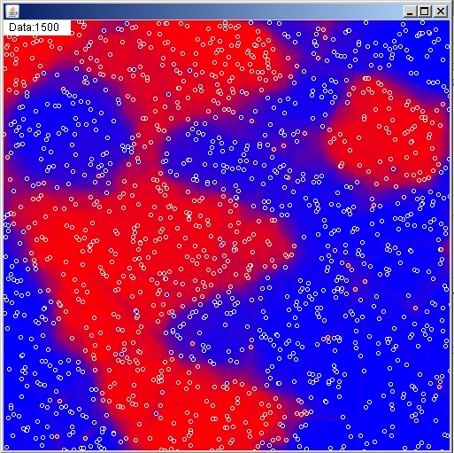
Just like the random forests we’ll be doing bootstrap aggregation and random feature selection (generating new random axes for each tree) to build forests of these new rotation trees. We’ll also be splitting rather deep, and generally not doing any tuning. We allow individual trees to overfit the subset of the data they’re given, and then those random errors tend to cancel out in aggregate. I’ve decided not to embed the complete code as it is a bit on the lengthy side, but a stand alone file of the entire algorithm can be viewed/downloaded here, and here’s a picture of the final algorithm in action:
Conclusion
Before we can call it done, I would like to mention that decision forests, and in fact any ensemble method, will be embarrassingly parallel. You can multi-thread the process very easily since the training of each individual model is independent from the others. Your average processor these days is a quad-core, so there’s a lot to be gained by making use of more than one core. I like to use 64 trees (varies by problem, experiment to see what works), but if you spawn a thread for each tree you’ll lose a lot of efficiency as your processor constantly switches contexts to try to avoid starving out any one thread for too long. Your best bet speed-wise is to spawn a set small number of threads up front (4 to 8 is good), and have each one train several trees.
The inductive bias of a decision tree is that the answer can be arrived at by asking a series of simple binary questions. However, allowing a large number of questions to be asked allows them to fit any arbitrarily complex edge boundary. Arbitrarily complex functions can lead to over-fitting, but that can be combated by building ensembles of trees called decision forests. By using rotation to ensure diversity and disrupt the blockiness bias of the standard tree we arrive at a classifier with an incredibly weak inductive bias. What this means in practice is that decision forests perform well when data is plentiful and relationships are complex.
In my experience the above rotation forest algorithm is one of the best performing techniques (both in accuracy and efficiency) for real classification problems. It does require a large amount of data to work well (thousands of data points), so a simpler function fitting algorithm may work better for small problems (dozens of data points). I am aware of algorithms that are competitive accuracy-wise, but they are typically much slower and always much more complex. In certain cases I have seen the standard Random Forest beat the rotation variety. Specifically, random forests are better at ignoring irrelevant variables, while a rotation forest will always mix all data into every axis making it weaker to junk variables. Typically though, rotation forests will edge out their random counterparts by just a little bit. In short: classification on large data-sets of fixed length numerical feature vectors is a solved problem and this is the solution.
If you don’t believe me, and you’re not yet savvy enough to test for yourself fear not. My next article will be on how to test and compare algorithms. Now that we’ve got a few tricks up our sleeves it’s time to pull down some real-world data-sets and see what really happens. I’d also just like to have a general framework for articles going forward. There are several more machine learning algorithms coming up in the queue that’ll need testing. I may take a detour into vision or numerical optimization first, though. We’ll play it by ear.
2 thoughts on “Decision Trees and Forests”