It’s important to know how well your models are likely to work in the real world. In this article I’ll be discussing basic testing procedures  for classification problems such as generating receiver operating characteristics and confusion matrices as well as performing cross validation. We’ll also take a look at the effect of over-fitting and under-fitting models.

Previous articles have talked about a handful of different ways to mathematically model data and use those models to make predictions. I’ve shown a few back of the napkin tests, basic curve fitting and the like, and those tests are fine for getting a sense of how an algorithm works or tracking down major bugs. They don’t, however, tell us how well an algorithm is going to work in “the real world”.

The real world is a messy place, or more specifically a noisy place. The measurements we use as inputs to our models are not perfectly accurate. The outputs may be partially random or dependent on factors we don’t consider. Sometimes the relationship between what we know and what we want to predict just isn’t in the data at all. In that case we won’t get good results no matter what algorithm we use. Validation is as much about testing your data as it is about testing your model.

In the “real world” the data-set will usually be given to you as part of the problem you’re tasked with solving. Since this blog is about machine learning algorithms we’ll be using existing data-sets from the UCI Machine Learning Repository. For our first set of tests we’ll use US congressional voting records from 1984. The problem is straightforward: given the voting  record of a congressman on 16 bills, predict which political party they belong to.

The first step is to split our data into two sets: a training set and a testing set. Since we’re interested in our ability to make predictions for future data it’s not very meaningful to test on the data we used for training. Especially since a lot of algorithms can build models sufficiently complex to effectively memorize the training data. Heck, nearest neighbor algorithms literally just memorize the training data.

How should you go about splitting your data-set into training and testing sets? First, I would recommend shuffling the order of your data points. It’s not uncommon for data-sets to be sorted on the output, which can completely throw off your modeling. For example: what if our congressional voting records data-set had all of the democrats at the top and all of the republicans at the bottom.  If we split in the middle we’ll end up training on a set of almost all democrats. We’ll get a model that just always predicts democrat. Then we’ll test it against the testing set of mostly republicans and get very low accuracy. We want to avoid sampling bias whenever possible, and the best way to do that is to draw random samples.

As for the relative sizes, the training set is usually much larger than the testing set (90/10 is common). In general we get a better model when we train on more data.  Each data point has some amount of random noise, and that randomness tends to cancel itself out as you average over more points. The only time this might not be the case is if we have ALOT of data with a relatively simple pattern.  If you’re target function is a parabola it’s not going to make a difference whether you train on 1,000 or 1,000,000 data-points.

Receiver Operating Characteristics

Ok, so we can download a data-set, split it into two parts, train on one of them and test on the other. Since we’re talking about classification today, what we’d ultimately get is a percentage accuracy: what fraction of our test population did we classify correctly. That’s fine for something like voting records, but let’s consider something else: a cancer screening. Maybe something like this one. This is a case where even if I probably don’t have cancer (my overall prediction comes back negative) if I have a non-negligible chance I still want to get further tests.

If we’re only looking at total accuracy we’re missing a big part of the picture. In the case of a life or death screening the difference between a misclassified healthy patient and a misclassified sick patient can be very significant. To resolve this discrepancy, rather than considering only two test outcomes (correct and incorrect) we consider four possible outcomes (true positive, true negative, false positive, and false negative). Considering our correct and incorrect separately depending on the true value we now have two accuracy values: sensitivity (aka true positive rate or recall) which is our accuracy for positive cases, and specificity (aka true negative rate) which is our accuracy for negative cases. In the cancer example above it’s clear that sensitivity is more important to us than specificity. If our specificity is low we may tell patients to get unnecessary tests, but if our sensitivity is low we may have more patients die of cancer.

So, given these concepts how can we build a model that prioritizes one over the other? Well, we can vary the threshold for what we consider a positives case, for instance we could say anyone with a 20% cancer risk should be checked instead of the default 50%. This isn’t a problem since almost all of the models we use output not just a yes or no prediction, but some sort of probability or numerical likelihood. We could run a test to see how well we do with a 20% threshold, but what if we’re not sure what threshold we want to use? This is where receiver operating characteristic curves (ROC curvers) come in.

A ROC curve is a graph of true positive rate vs false positive rate (which is 1-specificity) as threshold varies. Each point on the curve shows the results you could expect if you used a certain threshold, which can help us pick a threshold in the case where sensitivity and specificity are not equally important. The overall shape of the curve, specifically the area under the curve AUC (aka C-statistic) can be used to generally measure how well the model works for ALL thresholds.

AUC is equivalent to the probability that the classifier will rank a randomly chosen positive instance higher than a randomly chosen negative one.  It’s debatable how meaningful this is as a measure of classifier quality, but it is used quite frequently. If you know what threshold you want to use I’d say you’re better off using accuracy as the one true number of model quality, but for practical purposes if a model has higher AUC then it’ll probably have higher accuracy as well.

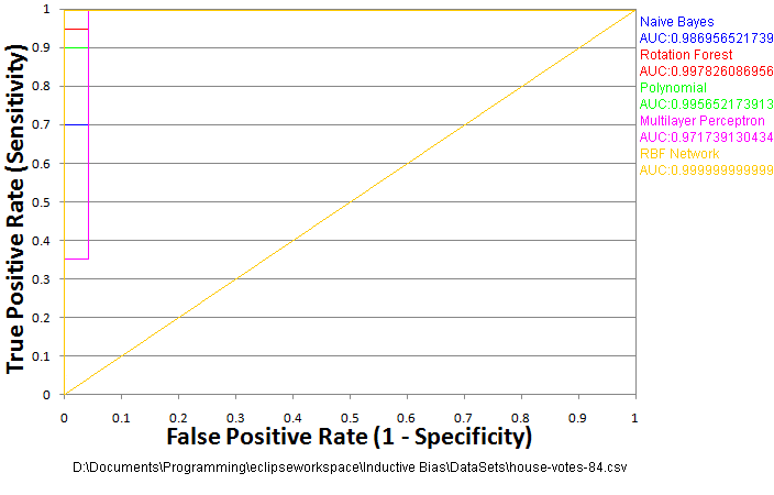
Generating a ROC curve doesn’t actually add much overhead to our testing procedure. We run the test once per test data point and store the model output along with that data-point. Then we sort all the test data points on their model output. We walk through the data points in order keeping track of true positives (TP), false positives (FP), true negatives (TN), and false negatives (FN) as we go . Use those to calculate the true positive rate, true positives/ (true positives+false negatives), and false positive rate, false positives/ (false positives + true negatives), periodically, which allows us to draw the line on the chart. Those four numbers (TP, FP, TN, and FN) can also be used to calculate a variety of other statistical measures if desired. Without further ado, let’s take a look at some ROC curves for our congressional voting data-set.

Cross Validation

That curve is a bit disappointing. There were only 435 data-points in that voting record set. I trained on 392 of them, which only left 43 for testing. It’s also a pretty easy data-set. None of the algorithms missed more than one. The RBF network didn’t miss any! That’s probably a fluke, but it’s hard to tell with so few test samples. We definitely need more test examples, but with so little data we don’t want to take any points away from the training either. The solution? Run more tests.

We could simply reshuffle the data and run the test again, averaging the results (repeated random sub-sampling validation). This isn’t a terrible idea, but there’s a better way. We shuffle the data once, then split it into k equal sized partitions. We run k tests using each partition as a test set for a run and all the other partitions as the training set for that run. Then we average the results of these k tests. This is called k-fold cross validation.  The advantage of k-fold cross validation over repeated random sampling is that every data point is guaranteed to be in a test set exactly once. Your tests are guaranteed to be diverse and thus, intuitively at least, more representative of what will happen with new data.

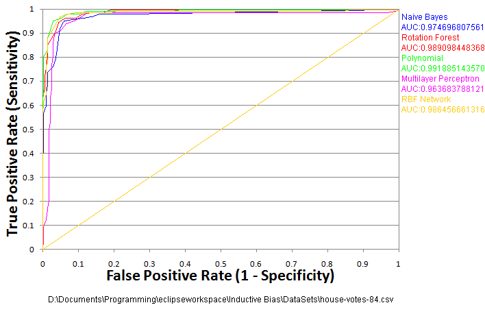
Ten is a pretty good and commonly used value for k.  You could do less, but then your training sets get smaller. On the opposite extreme you could do “leave one out validation”,  setting k equal to the number of data points and retraining with all but one point at a time to give your algorithm as much training data as possible. Ten-fold cross validation is what I’ll be using for the rest of this article.  Test results from cross validation are likely to be more accurate, reliable, and informative, but there is a down side. You have to run the test 10 times! It can be quite a pain for the impatient, especially if your algorithms are slow or you have a lot of data.  Let’s take another look at the congressional voting ROCs generated using ten-fold cross validation.

 Under-Fitting and Over-Fitting

That last ROC curve is a bit more informative, but it’s still a relatively easy problem. When it comes right down to it, it doesn’t really matter which of those algorithms you decide to use for that problem. Obviously, this isn’t always going to be the case, or we wouldn’t bother with anything beyond naive Bayes. Let’s take a look at a slightly more interesting problem. In this data-set we’re taking US census data, and trying to predict whether an individual’s income is above $50k/year.

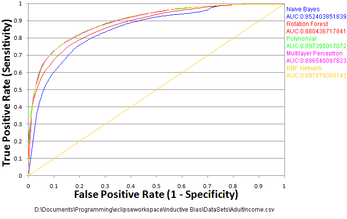
This data set has a number of categorical variables, which I’ve converted to numerical variables, but kept as single columns (probably not the ideal way to pre-process this data, but for the sake of example let’s say it came this way). There are columns like “occupation” where different numbers represent different occupations with no specific ordering. This information is certainly relevant for estimating income, but the relationship is also likely to be highly nonlinear. In a case like this it matters quite a bit which algorithm you choose.

The results here seem to show the two neural network algorithms (RBF network and multilayer perceptron) are just about tied with each other and the polynomial, while the rotation forest is a bit lower by itself, and the Naive Bayes is a bit lower than that. Why is that? Since three very different algorithms are essentially tied for first, it’s a relatively safe bet that’s about as good as you’re likely to get with this data (preprocessed in this way).

So, why is the Naive Bayes classifier performing worse than the others? The short answer: the model it builds (which is just 2 normal distributions, one for each class) is not complex enough to accurately model the underlying signal. It can’t model highly nonlinear relationships. It still does “ok”, but it’s never going to do as well as those other algorithms here because it’s under-fitting the data.

What about the rotation forest? The rotation forest algorithm here is the one presented in the previous article. It splits to an arbitrary complexity, so it doesn’t make sense to say it’s not complex enough.  However, this particular tree design has a weakness for fitting to “junk variables” that don’t actually matter. It’s actually fitting to noise in the training data that doesn’t generalize to the testing data. It’s not doing well because it’s over-fitting the data. However, unlike under-fitting, over-fitting can often be resolved by changing the parameters of the algorithm. In this case I can improve the results of the rotation forest simply by increasing the number of trees or reducing the tree depth.

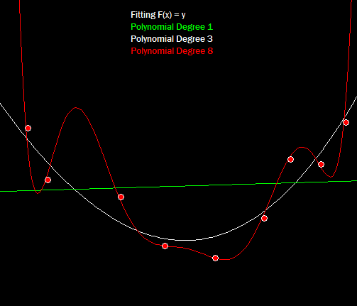
Under-fitting and over-fitting are related problems, and different algorithms deal with them in different ways. It’s possible to have both problems within the same algorithm just depending on the parameter settings. For example take a look at fitting polynomials to a small noisy data-set:

Confusion Matrices

Receiver Operating characteristics are great for binary classification problems, but they don’t really work for multi-class problems.  Let’s consider a new problem: recognizing hand written digits from 0 to 9. You could model this as 10 separate binary classification problems, and that often works well for training the models (the decision forest was trained that way below). The computer has no trouble dealing with 10 separate models, but it’s not very intuitive for a human to try to understand 10 separate ROC curves. It’s much more intuitive for us to look at a list of what is getting mixed up with what. A confusion matrix is just a grid of tallies where the first axis is which output was predicted and the second axis is the correct answer. Thus amounts along the diagonal (prediction = truth) are correct answers and everything else is incorrect.

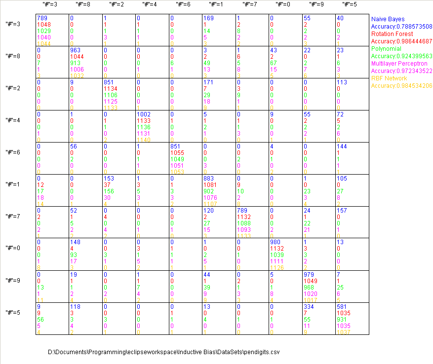
That last data-set has much more complex patterns than the previous two sets, and it’s also a problem where we expect a very high accuracy.  In this case I think it’s fair to say the naive Bayes classifier is no good at all. It only recognizes a little over half of the 5s. 78% accuracy on optical character recognition is hardly worth implementing. The polynomial also does quite poorly at 92% with the others clustered around 98%.

Conclusion

Accuracy and relative accuracy of different algorithms will vary wildly with different data-sets, so it’s always, always a good idea to run validation on a new model with an appropriately representative data sample before putting it into practice. It’s also a bit misleading to just look at accuracy as we’ve done thus far. Even just the 5 algorithms used in the examples in this article differ dramatically in their complexity to write and their run-times.

Pen Digit run-times in milliseconds:

Naive Bayes = 961
Rotation Forest = 88173
Polynomial = 2470
Multilayer Perceptron = 2055532
RBF Network = 240420

So, while the neural network models perform similarly accuracy-wise they are much slower and much more complex algorithms to code than the rotation forest. Decision forests are, in my opinion, the 20% effort that will solve 80% of the problems…As long as those problems don’t involve regression. We will get to the various neural network designs as well as a number of others (support vector machines come to mind), but we’ll have to cover the basics of nonlinear optimization before we can have any sort of meaningful discussion about those algorithms.

I’ve got quite a few potential articles in the pipeline both machine learning, computer vision, and a few other things with no particular required order. If there’s something specific you want to see let me know in the comments. Until next time, happy sciencing.