 Logistic regression uses a sigmoid (logistic) function to pose binary classification as a curve fitting (regression) problem. It can be a useful technique, but more importantly it provides a good example to illustrate the basics of nonlinear optimization. I’ll show how to solve this problem iteratively with both gradient descent and Newton’s method as well as go over the Wolfe conditions that we’ll satisfy to guarantee fast convergence. These are the prerequisites for the upcoming neural network articles!
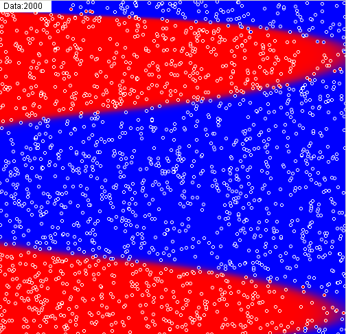
Today we’re talking about logistic regression, which despite having “regression” in its name is really only good for solving binary classification problems. The basic idea is to take a linear function on your input and sort of squish it into the 0 to 1 range by applying a sigmoid on the output. What you get is a function that is nearly 1 off to one side of a line/plane, nearly 0 off to the other side, with a continuous and smooth but usually quick transition. Training consists of trying to find the weights on that linear function that minimize the error on the final function.So, why bother adding this sigmoid, why not just use the linear function directly or a polynomial? We already know how to do that quick. The first reason is inductive bias. The inductive bias of the logistic function is that there exists a simple boundary that splits the 0s from 1s, and the further you get from that boundary the more confident you can be. Polynomials and lines will show soft boundaries where in reality there are hard ones. Additionally, polynomials have a nasty habit of shooting off in arbitrary directions at the edge of your measured data.
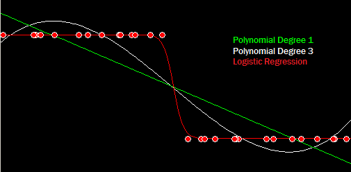
If you were to ask about a point just beyond the right edge of that picture the line(green) might predict -1, the polynomial (white) might predict +1, and the logistic regression(red) would predict something near but not quite 0. This is a binary classification problem with classes of 0 and 1, so the near zero prediction makes the most sense by far.
What happens when you add a polynomial to a polynomial? You get another polynomial of the same degree. What happens when you add a sigmoid to a sigmoid? You don’t get another sigmoid. You get something more complex. Actually, you can make functions of arbitrary complexity by adding a sufficient number of scaled and shifted sigmoid functions. This is essentially what’s going on in your basic multilayer perceptron. In short: if you can efficiently solve logistic regression problems then you’re well on your way to artificial neural networks.
Gradient Descent
Let’s take a look at the formula for our logistic regression model:
![]() Where x is an input vector, y is the output for that vector, s(x) is your standard sigmoid function, and w and b are the parameters of the model : the weight vector and bias respectively. The general approach to fitting a curve like this is to take a measure of total error on known data points (sum of squared errors is common) and minimize it. We can do this by setting the derivative or gradient of our error function to zero, and then solving the resulting equation to get the stationary points. The stationary points could be minimums, maximums, or saddle points, but if we have them all it’s a simple matter of measuring the error on each one and picking the one with minimum error.
Where x is an input vector, y is the output for that vector, s(x) is your standard sigmoid function, and w and b are the parameters of the model : the weight vector and bias respectively. The general approach to fitting a curve like this is to take a measure of total error on known data points (sum of squared errors is common) and minimize it. We can do this by setting the derivative or gradient of our error function to zero, and then solving the resulting equation to get the stationary points. The stationary points could be minimums, maximums, or saddle points, but if we have them all it’s a simple matter of measuring the error on each one and picking the one with minimum error.
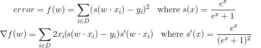
That’s what you get with a couple applications of the chain rule on our squared error measure where D is the data-set of known input/output pairs . I removed the “+b” from the first formula because the math is easier if we just stick a 1 on the end of each of our x vectors and append the bias value onto the end of the weight vector. Ok, now we just set that equal to zero and solve for w.
Yeah, that’s not happening. That equation is probably impossible to solve analytically. If it’s not impossible it’s at least really hard. We’re not going to be able to get a direct formula for the optimal weight vector to fit a logistic regression model to a data-set. We do have the error function though, which means we can tell how well any given weight vector fits our data. We can also calculate the gradient of the error which always points in the direction of steepest ascent. Since we want to decrease error we’re interested in the direction of steepest descent which is actually the negative of the gradient.
The basic idea behind gradient descent is to walk your parameters “downhill” in your error function until you can’t anymore. Once your gradient becomes sufficiently close to zero then you know you’re at a stationary point, and since you got there by going down as much as possible you can be reasonably certain that it’s a minimum (it could be a saddle point but it’s very unlikely). Gradient descent can be used to solve a wide variety of model fitting and other problems. If you can come up with a formula for how well a model fits and you can take it’s derivative then you can use gradient descent to fit the model.
Unfortunately, the gradient doesn’t tell you everything. It tells you a direction you can move in to improve, but it doesn’t tell you how far to go in that direction. It also doesn’t tell you anything about where to start looking, and since you’re only guaranteed to find a local minimum, where you start can be pretty important. Let’s start there…ha.
Initial Point
Even if we have a method to iteratively improve upon the parameters of a model, we still have to have a starting point to improve upon. We could start at all zeroes or random numbers in some range. That is something I do occasionally. In this case we can do better, and if we can get closer with our initial guess then it will take less iterations to converge and be more likely to converge to the best solution. Gradient descent takes us to the bottom of a valley, but we’ll only get the best answer if we start in the lowest valley.
There’s no general method of getting a good initial guess. In the case of logistic regression I’ve noticed that if you apply the inverse sigmoid function to both sides of the model function you get a linear least squares problem, which I covered in a previous article. The least squares result without the sigmoid is definitely not the same as the least squares result with it, but it could be a reasonable starting point. I think that’s a bit overkill for this though, so let’s go with something simpler. I’m going to find the center (centroid) of the positive cases, make that 0.75, and the center of the negative cases, make that 0.25, and then just have the function increase in the direction from negative to positive.
Then alpha and the bias can be found by intersecting those two lines with a simple formula derived from Cramer’s rule. This doesn’t necessarily find a great fit, but it cheaply finds one that’ll get generally higher outputs for positive cases than negative cases. It gets us in the ball-park.
Determining Step Size
We’re in the ballpark and we know which direction to go to make improvements, now we need to know how far to go on each step. If we take steps that are too big we risk repeatedly jumping over the minimum. We can guarantee we get close to the minimum if we always take small steps (this is what most algorithms that have a “learning rate” are doing), but taking small steps requires we take more steps, so it’s going to take a lot longer. We need some way to take larger steps when possible, but still guarantee that we’ll reach the minimum.
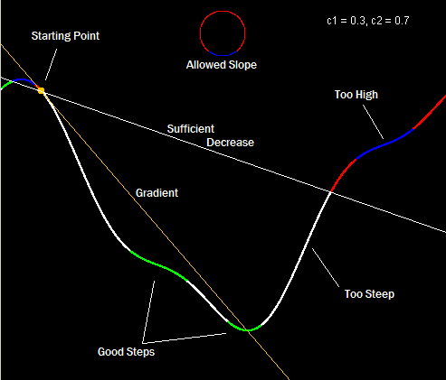
The Wolfe conditions are a set of conditions on step-sizes that if met guarantee convergence for repeated descent direction steps. I’m not really going to go into how they’re derived or proving that they work, but the basic idea is that if the new position decreases the error by enough you can guarantee convergence and if you also also reduce the steepness of the slope at each step then you’ll converge faster.
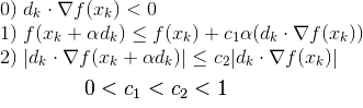 Xk and dk are the starting position and search direction respectively. Once you’ve selected a search direction, determining the step-size alpha becomes a 1-dimensional problem. Equation 0 (which isn’t actually part of the Wolfe conditions) is the mathematical way of saying you have to pick a direction that goes downhill in your error function. Gradient descent always selects the negative of the gradient, which obviously works, but you can guarantee convergence for any generally downward direction. Equation 1 says the new point you’re moving to has to decrease error by a certain fraction (c1) of what you’d get moving along the tangent line. Equation 2 is the strong Wolfe condition on curvature which says the slope along the search direction has to get flatter by a certain fraction (c2). Maybe this picture will help:
Starting from the yellow point in the upper left corner (
")

You may notice there are two acceptable regions or more importantly that there are acceptable regions. If your search hits anywhere in those areas then you can accept the point and stop the line search. Why do we bother accepting any of those suboptimal points? The short answer is that searching is expensive and the line-search is just a sub-problem. Usually after we do a line-search we’re going to immediately calculate a new search direction and do another line-search. C1 and C2 affect the strictness of our requirements and can be used to tweak how much time we spend searching a direction vs calculating new directions.
I’ve told you how to tell if a step-size in a line-search is good, but I haven’t actually told you how to calculate one. There is more than one way to do this, but in the interest of simplicity a binary search works just fine. Start by defining a region you expect the step-size to fall in. The minimum alpha should be 0 (you have to go forward but step can be arbitrarily small) and the maximum is a somewhat large arbitrary number say 100 or 1000. Your step is alpha times -gradient, so if you’re expecting an unusually small gradient your max alpha may have to be bigger.
To search you sample an alpha in the middle. If it satisfies the conditions you’re done. If it’s too far then set max alpha to the current alpha and sample a new alpha in the middle of the new region. Similarly if it’s not far enough then set min alpha to the current alpha and sample a new alpha in the middle of that new region. You can tell whether it’s too close or too far based on which condition is violated. If error doesn’t decrease enough or the function is now sloping upward then you’ve gone too far. If it’s too steep and still sloping downward then you haven’t gone far enough.
Logistic Regression
Once you have all of the parts the main gradient descent loop is very simple. The hardest part of applying these techniques to a problem is in formulating the error function and gradient. I kind of glossed over the gradient calculation above. What if I made a mistake? Well, it’s possible (and generally a good idea) to approximate the gradient numerically and see if it’s similar. Numerically calculating the gradient is just a matter of taking the slope along each axis over a small length. It’s a good way to catch a bug in your analytically calculated gradient, but in subtracting two very close numbers you lose a lot of your machine precision and the numerical gradient requires 2*(dimension of input vector) evaluations of the error function making it usually much slower than calculating the analytical derivative. In short: suck it up and do your calculus.
Newton’s Method
Above is the bare minimum you’d need to reasonably solve an unconstrained nonlinear optimization problem, but it’s by no means the only way. Optimization, finding minimums or maximums, is essentially the same as finding a zero or root of a function (that function being the gradient of your error). We’ve had good techniques for doing that for literally hundreds of years, and one of the best is Newton’s method.
![]() The geometric reasoning behind Newton’s method is to use the derivative to build a tangent line at your initial guess, and then intersect that with the x-axis to get a new guess for the root of the more complex function. This isn’t always guaranteed to work, but given the right conditions and a good initial guess it converges quadratically, which is to say very quickly. As an example let’s look at calculating the square-root of 2. We want to find x so that x^2 = 2. This is the same as finding the root for f(x) = x^2 – 2. I know it’s pretty close to 1.5, so that’ll be our initial guess.
The geometric reasoning behind Newton’s method is to use the derivative to build a tangent line at your initial guess, and then intersect that with the x-axis to get a new guess for the root of the more complex function. This isn’t always guaranteed to work, but given the right conditions and a good initial guess it converges quadratically, which is to say very quickly. As an example let’s look at calculating the square-root of 2. We want to find x so that x^2 = 2. This is the same as finding the root for f(x) = x^2 – 2. I know it’s pretty close to 1.5, so that’ll be our initial guess.
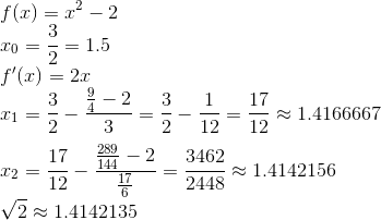
Two iterations of Newton’s method takes us from being within 0.1 of the correct answer to to being within 0.00001. A binary search would take over a dozen iterations to improve accuracy by that much. That’s why we care, so how do we apply this to general optimization problems?
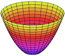
The main wrench in directly applying Newton’s method to optimization is that we’re interested in functions of multiple variables. This means the gradient, which is what we’re finding the root of, is a vector, and every element of it needs to go to zero. It gets worse, since f(x) above is the gradient, f'(x) above is the gradient of the gradient, also known as the Hessian, which is a matrix of the second derivatives of our error. Geometrically, using Newton’s method for minimization is like building a quadratic approximation, a paraboloid, of our error and then jumping directly to it’s lowest point.
There are a few other problems. Newton’s method requires certain conditions to work, conditions that we can’t in general guarantee. Even when it does work it won’t necessarily go to a minimum of our error. Depending on where we start it could just as easily take us towards a maximum or saddle point. This isn’t actually a problem though because we have the Wolfe conditions. We can use a vector pointing toward the Newton iteration as a step direction. If it’s a descent direction, and we do our inexact line-search then convergence is guaranteed. Ideally, the raw Newton step (with a step-size of 1) will satisfy the Wolfe conditions causing the inexact line-search to exit immediately without having to check any other points. If Newton’s method turns out not to be a descent direction then we can fall back to gradient descent for that step.
We still have to deal with the many variables. We can do this by rearranging the basic formulation. First off we’re interested in the direction to go in (
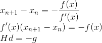 H and g are the hessian matrix and gradient vector respectively both calculated for the current x , while d is the search direction we’re trying to find. At this point the problem of finding the Newton step reduces to solving a system of linear equations, which I covered how to do efficiently with a Cholesky decomposition in my article on linear least squares. If you remember from that article the Cholesky method has a few requirements of it’s own. Specifically the matrix (H in this case) must be symmetric (
Positive definite in terms of the Hessian matrix means that our quadratic approximation is a paraboloid opening upwards. It conveniently happens that this is the same requirement to get a Newton step that’s pointing towards a minimum. So if our H matrix isn’t positive definite then our Newton step is junk anyway, and we can just stop and switch to gradient descent in that case. How do we tell if our H is positive definite? Attempt to take the Cholesky decomposition.
The basic Cholesky decomposition has square-roots in the formulas along the diagonal. If negative numbers pop up under them then it can be considered to have failed, and thus the original matrix wasn’t positive definite. If you’re using the LDL variety described in my previous article to avoid computing those square-roots then you can check if the square-roots would have failed by checking for negative numbers in the D matrix . If all of the numbers along the diagonal D matrix are positive (zeros are also bad) then your Newton step is useful and you’ll succeed at calculating it with the Cholesky decomposition.
I’m not going to embed code for Newton’s method in the article because it’s pretty long and mostly repeated matrix code from the other article, but it’s all commented in the final code for this article, which you can check out on GitHub.
Logistic Regression 2
Let’s go back to our logistic regression use-case for a moment and take a look at calculating one of those Hessian matrices.
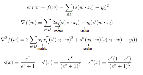 The s(x) sigmoid function is a common single variable function. You can get its derivatives by politely asking Wolfram Alpha. Most of the work in calculating the main derivatives is just repeated applications of the chain and multiplication rules. It’s a bit messy, but it’s basic college calculus, and you can find other tutorials on that if you need them.
However, I do want to take a moment to talk about the matrix and vector components. It’s common in literature to see vectors treated as column matrices of width 1. The inner dimensions have to match in matrix multiplication, so if you want to multiply a 5×1 matrix by another 5×1 matrix you can’t do it directly. You have to transpose one of the matrices. If you transpose the first one then you multiply a 1×5 and a 5×1 and you get a 1×1, which is a scalar that’s equal to the dot product of the two vectors. (x ^t * x is the same as x dot x in common notation).
But you can also multiply two vectors by transposing the second one. Then you’d multiply a 5×1 and a 1×5 and get a 5×5 matrix where 
Much like with the gradient it’s generally a good idea to check your hessian against a numerical approximation. Also, like the gradient it’s much better to use the analytical solution in the final code for this case. In particular the part of the Hessian function that has all the exponents and divisions is separate from the matrix part, and thus only needs to be calculated once for each data-point and not for every element of the matrix.
Much like the linear least squares method this logistic regression algorithm can also be expanded to use polynomials or other functions by preprocessing the input vectors. Since what we’re solving for in the optimization is the weight vector, the data-points are treated as constants, and preprocessing them doesn’t affect any of the calculus. One minor caveat is that the initial guess doesn’t make quite as much sense in that case. If your data has been normalized (shifted to have a mean of zero and scaled to have a standard deviation of 1) then starting at weights of all zeroes may work better than the initial point described earlier.
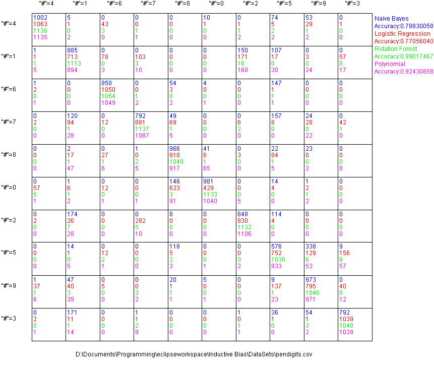
I also ran that “pen digits” character recognition data-set I used in the validation tutorial. I didn’t do any preprocessing, so it’s just using linear separators, and the performance is pretty close to that of Naive Bayes. Both methods are limited by the low complexity of their models.
Conclusion
Logistic regression is a pretty simple model relative to other machine learning techniques available, and I can’t think of a problem off the top of my head where it would be my first choice. I mainly covered it because it’s a good example for discussing general optimization and because I’ve often seen it implemented poorly. I use that little color matching app pictured above as a generic sanity test for my algorithms. It takes about 25 milliseconds using Newton’s method but over 4 minutes using just gradient descent.
The main purpose of this article was to familiarize you with gradient descent, Newton’s method and Wolfe condition line-search. Those ideas pop-up a lot in machine learning as well as computer vision and other places. These are the basics, but they’re not all there is to nonlinear optimization. We didn’t talk at all about how to deal with constraints, and I didn’t even mention my favorite optimization method L-BFGS. Still, if you can understand what’s presented here it opens up a lot of previously closed doors. If you can formulate a measure of error and take it’s derivatives then you can efficiently minimize that error, and that’s kind of a big deal.
Now that optimization basics are out of the way, we’re in a good spot to start talking about a variety of more complicated things. Neural nets are a big one, and there are several types of those I want to discuss….eventually. In the short term I’d like to switch gears and do a series on computer vision techniques such as optical flow, 3D reconstruction, and super resolution. I’ve purchased a nice little aerial drone that I think will be great for getting interesting imagery for those algorithms. Stay tuned. It should be fun.
One thought on “Logistic Regression and Optimization Basics”