Today we’re talking about linear least squares curve fitting, but don’t be fooled by the name. I’ll show how to use it to fit polynomials and other functions, how to derive it, and how to calculate it efficiently using a Cholesky matrix decomposition.

We’ve got one set of input vectors where each one also has a corresponding output vector, and we’ve got a second set of input vectors that don’t yet have outputs. We want to learn the relationship between inputs and outputs using the first group and then use it to predict the outputs for the second group. This is your classic supervised learning problem, but unlike the Naive Bayes algorithm in the last post, this time we want to get actual numbers, not just which class the input belongs to.  We can do this by fitting a line or a polynomial to our data, and both of these functions can be fit using linear least squares.

Derivation

Let’s say we have an input vector X, and we want to find the linear function that best predicts an output scalar y. That is y = C*X (C dot X) where C is the vector of coefficients we’re solving for. In reality we have several X’s each with it’s own y, so X becomes a matrix with each row being a single input vector and Y becomes a vector of all of the outputs for each input vector.

If the number of training points is exactly the same as the length of an input vector of a training point then the X matrix will be square and all we have to do is solve the resulting system of linear equations for the C vector.  Barring some sort of matrix singularity, this C vector will produce a function which goes perfectly through all of the training points. Realistically, the number of training points (think thousands) will far exceed the number of input variables (think dozens). It’s usually not possible to pick a C which perfectly hits every training point, so we have to pick one that fits them as well as possible. In the case of least squares this means picking the one that gets the least sum of squares of the error for each training point, hence the name of the algorithm.

That is, we want to find the C vector that gives the minimum value if we multiplied it by our X matrix and subtracted the desired output and squared it. How do we do this? It’s simple calculus. Remember Fermat’s theorem? Probably not by name, but it’s the thing where you set the derivative equal to zero to find minimums and maximums.

 

This looks exactly like our previous formula except with an X transposed prefacing each side. If X is an n by m matrix where n is the number of data points and m is the length of an input vector then X^T * X will be m by m and X^T * Y will be m by 1. This is good because it means the system of equations we need to solve to find C is square, so it has a unique solution, but its size is also independent of the number of training  points. In addition any matrix of the form X^T * X has a few other useful properties we can take advantage of. Specifically, it is symmetric (that is Mij = Mji), and it is positive definite (that is a^T X a > 0 for all a). The savings from symmetricness is fairly straightforward: almost half of the matrix doesn’t need to be calculated or considered because it’s going to be the same as the other half. The positive definiteness guarantees that out solution is a minimum, and it turns out to be a requirement for the method we’ll use.

Solving the System of Equations

At this point we have a system of linear equations which we could solve using your generic linear algebra class Gaussian elimination. However, that’s not a very good idea for two reasons: it’s unstable and it’s slow.  Unstable in this case meaning the loss of precision from using computer arithmetic will be compounded by the operation, and slow meaning, well, slow.

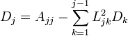
There are two algorithms I consider good candidates for solving this problem: Cholesky decomposition and QR decomposition.  Both of these techniques work by breaking the matrix into two matrices that produce a problem which is easier (i.e. computationally cheaper) to solve. The primary difference being that the Cholesky runs on the already calculated X^T*X, while the QR computes its factorization of X^T*X directly from X itself.  The QR is a bit more stable since some accuracy is lost when computing X^T*X, but the Cholesky is faster and in my experience plenty stable enough. We’ll be using the Cholesky today. Let our X^T * X be A, and the Cholesky decomposition is arranged as follows.

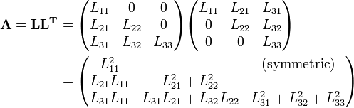
The important thing to note here is that L is lower diagonal. This means solving a system of equations with it is as simple as back-substitution.  I’m not going to go much into the derivation of the decomposition itself, but suffice to say you could set the multiplied out form equal to A and work out the formulas. One of which looks like the following:

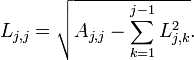
If you looked at this and immediately thought “well, that seems silly to take the square root and then just end up multiplying it back together in the next step” then congratulations you’re smarter than I am. I’m pretty sure I had to be told that it’s possible to factor out the diagonal terms in a separate matrix D and avoid those square-roots entirely without really adding any extra work. This form is called the LDL decomposition, and it looks something like this:

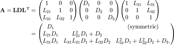
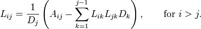
This is what I recommend using to solve linear least squares problems. Calculating the decomposition is as simple as just plugging these formulas into your code, but you do need to be a bit careful as both formulas make use of earlier calculations of each other. You have to walk through and calculate the D’s for each row at the same time you calculate a row of L.

double[][] L = new double[inputs][ inputs];
double D[] = new double[inputs] ;
//for each column j
for (int j = 0; j < inputs; j++){
  D[j] = XTX[j][j];//calculate Dj
  for (int k = 0; k < j; k++){
    D[j] -= L[j][k] * L[j][k] * D[k];
  }
  //calculate jth column of L
  L[j][j] = 1 ; // don't really need to save this but its a 1
  for (int i = j + 1; i < inputs; i++){
    L[i][j] = XTX[i][j];
    for (int k = 0; k < j; k++){
      L[i][j] -= L[i][k] * L[j][k] * D[k];
    }
    L[i][j] /= D[j];
  }
}

Alright, so you’ve got L and D factors of your X^T*X, but what you really want to do is solve for C back in the original equations. This can be achieved by solving the system of equations with each matrix from the outside to the inside. Since L is triangular, forward substitution can be used to solve for what D(L^T)C should equal. Since D is diagonal a few divisions will give us what (L^T)c should equal. Finally, a step of backward substitution gives us the final C.

Original equation

stick in the LDL and rename RHS

solve this with forward substitution

solve this with a few divisions

Solve this with backward substitution.

public double[] solvesystem(double L[][], double D[], double XTY[]){
  //back substitution with L
  double p[] = new double[XTY.length] ;
  for (int j = 0; j < inputs; j++){
    p[j] = XTY[j] ;
    for (int i = 0; i < j; i++){
      p[j] -= L[j][i] * p[i];
    }
  }
  //Multiply by inverse of D matrix
  double q[] = new double[p.length] ;
  for (int k = 0; k < inputs; k++){//inverse of diagonal
    q[k] = p[k]/D[k];//is 1 / each element
  }
  // forward substitution with L^T
  double c[] = new double[q.length];
  for (int j = inputs - 1; j >= 0; j--){
    c[j] = q[j] ;
    for (int i = j + 1; i < inputs; i++){
      c[j] -= L[i][j] * c[i];
    }
  }
  return c ;
}

Improvements

Huzzah, we have achieved linear least squares. The name linear least squares is a bit misleading because it’s linear in the parameters not the input variables. In actuality you can do pretty much whatever you want to the input variables as long as you do the same thing before training that you do when you apply the function.  Linear least squares will find the best fit linear combination of whatever you feed into it. By far the most common thing I see done is to use polynomials of the data. When given the inputs [a b c] instead of passing them in raw, pass something like [1 a b c a^2 b^2 c^2]  then performing the linear least squares fit gives you a quadratic polynomial fit*.

There is one more significant improvement that can be made to this algorithm before we can call it a day.  The LDL decomposition is the same size as X^T*X, and its construction never references  an element of X^T * X for which the L element has already been computed. This means we can compute the entire decomposition in place in a single matrix. We can place the D over top of the diagonal of the L (which is all 1’s so we don’t need to save it), and then we proceed to write L and D right on top of where X^T*X used to be.  Similarly, we don’t need to use new vectors to store each of our intermediate substitution steps. We can write p,q, and even c right over top of where X^T*Y used to be.

This won’t save us very many operations, but it can have a significant impact on performance because of the way computer cache works. By accessing less data and accessing it in a very structured sequential way we increase the chance that what we want is already in cache near the processor, and this reduces the number of times our program has to go out to main memory to find what it needs. So without further ado, here’s the final version of the code which fits a least squares polynomial from multiple inputs to multiple outputs using an in-place LDL decomposition.

//performs a least squares fit of a polynomial function of the given degree
//mapping each input[k] vector to each output[k] vector
//returns the coefficients in a matrix
public static double[][] fitpolynomial(double input[][], double output[][], int degree){
   double[][] X = new double[input.length][];
   //Run the input through the polynomialization and add the bias term
   for (int k = 0; k < input.length; k++){
      X[k] = polynomial(input[k], degree);
   }
   int inputs = X[0].length ;//number of inputs after the polynomial
   int outputs = output[0].length ;//number of outputs
   int datapoints = X.length ;//number of data points
   //calculate X^T*X
   double[][] XTX = new double[inputs][] ;//XTX is symmetric
   for (int i = 0; i < inputs; i++){//so we only have to
      XTX[i] = new double[i+1] ;//build the lower triangle
      for (int j = 0; j <= i; j++){
         for (int k = 0; k < datapoints; k++){
            XTX[i][j] += X[k][i] * X[k][j];
         }
      }
   }
   //calculate the LDL decomposition in place with D over top of the diagonal
   for (int j = 0; j < inputs; j++){
      for (int k = 0; k < j; k++){//D starts as XTXjj then subtracts
         XTX[j][j] -= XTX[j][k] * XTX[j][k] * XTX[k][k];//Ljk^2 * Dk
      }
      for (int i = j + 1; i < inputs; i++){//L over the lower diagonal
         for (int k = 0; k < j; k++){//Lij starts as XTXij then subtracts
            XTX[i][j] -= XTX[i][k] * XTX[j][k] * XTX[k][k];//Ljk^2*D[k]
         }
         XTX[i][j] /= XTX[j][j];//divide Lij by Dj
      }
   }
   double[][] matrix = new double[outputs][] ;
   //perform the substitution for each output separately
   for (int o = 0; o < outputs; o++){
      double[] XTY = new double[inputs];
      //multiply this output column by X^T to get RHS of least squares problem
      for (int j = 0; j < inputs; j++){
         for (int k = 0; k < datapoints; k++){
            XTY[j] += output[k][o]* X[k][j];
         }
      }
      //in-place forward substitution with L
      for (int j = 0; j < inputs; j++){
         for (int i = 0; i < j; i++){
            XTY[j] -= XTX[j][i] * XTY[i];
         }
      }
      //Multiply by inverse of D matrix
      for (int k = 0; k < inputs; k++){//inverse of diagonal
         XTY[k] /= XTX[k][k];//is 1 / each element
      }
      // in-place backward substitution with L^T
      for (int j = inputs - 1; j >= 0; j--){
         for (int i = j + 1; i < inputs; i++){
            XTY[j] -= XTX[i][j] * XTY[i];
         }
      }
      //copy into final matrix row for this output
      matrix[o] = XTY;
   }
   return matrix ;
}


//applies a polynomial built with the fitpolynomial method
public static double[] applypolynomial(double input[], double matrix[][], int degree){
   double[] i = polynomial(input, degree);//apple the same polynomial
   double[] o = new double[matrix.length];
   for (int j = 0; j < o.length; j++){//multiply by the matrix
      for (int k = 0; k < i.length; k++){
         o[j] += matrix[j][k] * i[k];
      }
   }
   return o;//return result
}


//Creates a new input vector which is a 1, and each input raised to integer powers up to degree
//when called with degree=1 this simply adds a bias value to the input vector
//otherwise it creates a separable polynomial of the given degree
public static double[] polynomial(double[] input, int degree)
{
double[] output = new double[1 + input.length * degree];//1 is for the constant
int i = 1, k, j;
for (k = 0; k < input.length; k++){
    for (j = 1; j <= degree; j++){
        output[i] = (double)Math.pow(input[k], j);
        i++;
    }
}
output[0] = 1; //constant
return output;
}

Conclusion

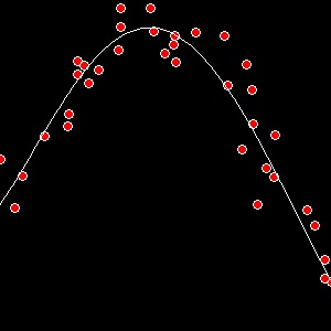
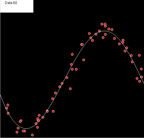
This time I took the liberty of running a few tests to help visualize the results. Here’s a            y = f(x) example with a degree 5 polynomial:

And here’s an f(X,Y) = (R,G,B) test where the polynomial is fit to make the background match the color of the points:

The inductive bias of a linear least squares fit curve is that the function you’re trying to match is a linear combination of the functions you pass in.  The complexity of the resultant function will always be exactly what you select up-front, which can be a good or bad thing. Using higher degree polynomials can create unpredictable wiggles between training data, while using lower degree polynomials may not be complex enough to fit your desired function. In either case the resultant function is likely to be wildly inaccurate outside the range of your training data.

Polynomials are inherently smooth. This often works in our favor when dealing with noisy data in that simply fitting the polynomial will act to give us a smoother representation of our data, but it does mean that polynomials may return a soft boundary where in fact a very hard edge exists.

Any algorithm that works by way of minimizing squared error will have a weakness to outliers. For instance if you have 10 points with the same input with 9 outputting 0’s or 1’s and one outputting 10,000, the resulting least squares function will return 1,000. Often in a case like this it would be better to ignore the wildly differing point, and if you’re dealing with data where you expect to have some points that are just flat out wrong you may want to consider a different technique.

Even considering all the downsides, fitting a polynomial is often one of the first things I try when given a new data-set. It’s fast, it’s easy, it works on both classification and regression problems, and I can look at the polynomial itself to get an idea of the basic relationships between variables. It’s rarely going to give you the highest possible accuracy, but I’d bet on it over Naive Bayes any day of the week.

* Regardless of technique, stability of a polynomial fit is going to depend heavily on the range of your data. I highly recommend normalizing your data points before attempting anything above a quadratic polynomial. This is explained briefly in the article on decision forests.