 Optical flow is the apparent motion of objects across multiple images or frames of video. It has many applications in computer vision including 3D structure from motion and video super resolution. In this article I illustrate one specific technique for calculating sub-pixel accurate dense optical flow by matching continuous image areas using optimization techniques over bilinear splines.
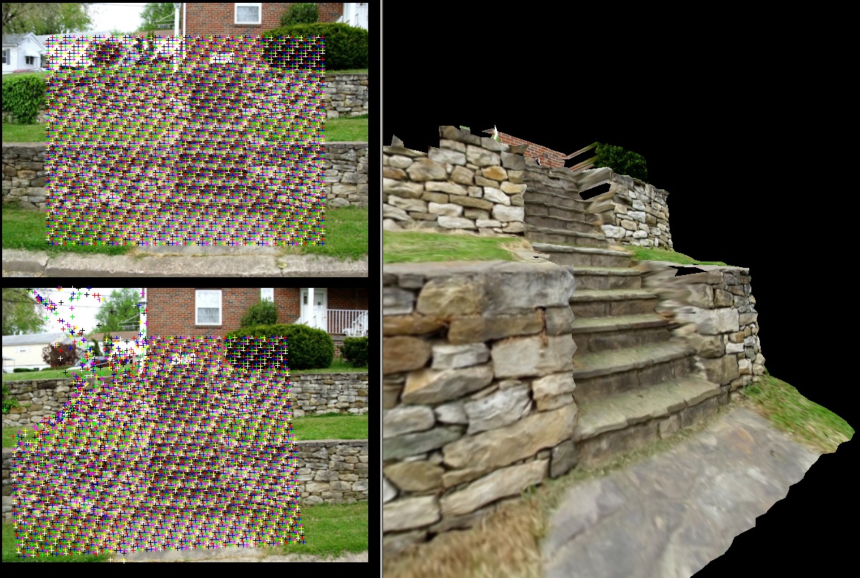
Consider the problem of 3D reconstruction from images: given two images of the same scene how can we determine the depth and 3D structure of the objects in the scene? If the images are separated horizontally and lined up like two eyes then this is a traditional stereo vision problem. Determining the depth of a pixel in the first image requires searching along a horizontal line in the second image and finding the matching pixel then the depth is some constant divided by the pixel distance between the two matching points.
Most of us don’t have a precisely aligned multi-camera rig lying around for taking 3D pictures. So what if we use pictures taken from the same camera in slightly different, not rigorously aligned, positions. Can we still get a 3D reconstruction of the scene? Spoiler: yes, but it’s quite a bit more difficult. We now have two problems we have to solve: we have to find matching points between the images, same as before, but we also need to figure out where each picture was taken from. There’s one more issue: without aligned cameras matching points are no longer guaranteed to lie on the same horizontal line. Without knowing where the camera was located a point’s match could be anywhere in the image, and without having point matches we can’t figure out where the cameras were located.
There are a few ways to approach this problem. You could use a feature detector. Find a few (5 to 10) key feature points in each image and then match among those. Using those matches you could rectify the images (i.e. align the images in software). Then dense matching could be done with a normal stereo vision search along horizontal lines (I may cover this approach at some point). Alternately, you could just do the search for matches over the entire image without making use of specific camera location information. This approach is called optical flow, and calculating it is the topic of this tutorial.
Optical flow is the relative motion of pixels from one image to another. It makes the most sense with frames of video, but it can be used with any images that are reasonably close together. How close the images have to be depends on what algorithm you use to calculate the optical flow. Of which there are many complex examples. Far more than I could or would want to cover on this blog. The algorithm I’ve chosen to cover is one I designed for video super resolution. In video super resolution the resolution and quality of a frame of video is increased by making use of information from neighboring frames which must be aligned in this case by using optical flow.
The method contained in this article is not the fastest optical flow algorithm, and it’s certainly not the most resistant to poor image conditions, but is among the most precise. It consistently aligns image points with sub-pixel accuracy, which is to say at a higher resolution than the images themselves (2x-3x is possible but it depends heavily on starting image quality/resolution). That’s a requirement for video super resolution. It isn’t a requirement for 3D reconstruction, but it does mean higher detail reconstructions.
Additionally, by making rather strong assumptions about continuity the method generates a very dense set of matches. Any pixel in the covered region is guaranteed to have a match (although it’s not guaranteed to be accurate), which leads to 3D models with relatively few holes and video enhancements covering almost the entire frame. In short the technique covered here is kind of slow and prone to failure (although that may just be the nature of optical flow), but in cases where it does work it produces very high quality results . Let’s talk about how to do it.
Bilinear Sampling and Interpolation
We’re developing a method to match points at higher than pixel resolution, so we need to be able to sample image colors at higher than pixel resolution. The easiest way is to assume color changes continuously and interpolate between the 4 nearest pixels to the point of interest. Bilinear interpolation is the simplest way to interpolate between 4 points. It’s cheap to calculate and it produces a smooth gradient which is ideal for the match optimization we’ll be doing.
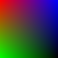
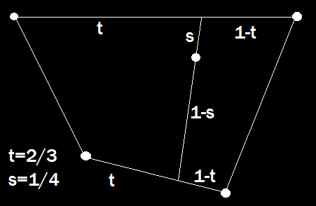
Bilinear interpolation is just a one dimensional linear interpolation applied to another set of two one dimensional linear interpolations. It has two parameters I’ll call s and t. In the case of interpolating pixel color t is the fractional part of of the x coordinate in the image and s is the fractional part of the y coordinate in the image. Thus if we want the color at position (6.7, 5.4) we would interpolate between the pixels at A=(6,5), B=(7,5), C=(6,6), and D=(7,6) with t= 0.7 and s =0.4 using this formula:
![]()
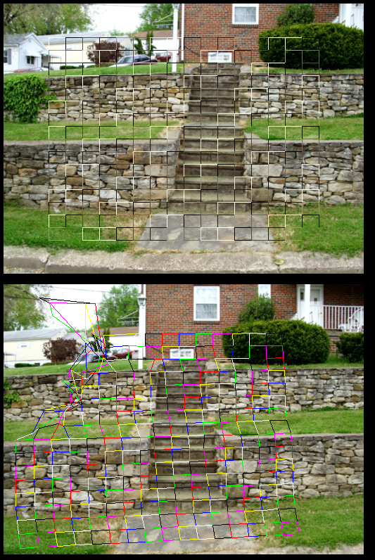
Bilinear interpolation is useful for more than just interpolating pixel color though. It can also be used to generate points over a quadrilateral. We still have 4 control points and we still have s and t ranging from 0 to 1, but instead of interpolating RGB color vectors we’re interpolating the (x,y) coordinates of our control points. We can vary s and t to create a set of points that cover the quadrilateral. For instance if we step both s and t by 0.1 we can get a 10×10 grid of points distributed over the entire quadrilateral. We can sample the color at those points (using bilinear interpolation as above) and generate a simple 10×10 image of what’s underneath that quadrilateral.
 If we use two such quadrilaterals, one on each image, and generate a 10×10 sample of each we can take the difference of these two samples to see how well the patches match. This measure of patch similarity is the core of the objective function we’re going to use for optical flow. We have a few control points at the corners of the patches that we move around to optimize how well the image areas under the patches match between the images.
Optimization
We have a measure of how well patches match across the images. In order to match over the entire image we need to cover it in these patches. For this algorithm I make a very strong assumption about continuity: that the function of optical flow is completely continuous, which is equivalent to saying the the depth field of the image is continuous and both images show exactly the same surfaces. This isn’t likely to be completely true, but it will usually be “mostly true” and the algorithm will “mostly work” in the continuous regions. It will fail horribly in cases where the images show different objects, but those cases are impossible anyway. We can’t match objects that aren’t in both images.
 We have our objective function: the difference between all the corresponding patches, but if you’ll recall from the optimization article we also need the derivative (and ideally the second derivative) if we want to optimize it in a reasonable amount of time. This is a rare case where it doesn’t make sense to calculate those analytically. Calculating the rate of change of bilinearly interpolated colors as patches shift past each other would be very difficult and probably slow, so we’ll use numerical derivatives this time.
We could naively shift each variable and reevaluate the entire objective function, but we can do much better by realizing that each control point only ever affects the 4 patches connected to it. The values of all the other patches will remain constant so long as we only change that control point, and thus would cancel out in the subtraction of the numerical gradient, so we don’t need to compute them. This problem becomes much easier if we only consider optimizing a single control point at a time.
Operating on only a single control point is equivalent to setting all other values in our step to 0. If we have a descent direction in the nonzero variables then it will still be a descent direction with the zeroes, and as long as we do eventually optimize over all variables (by looping through every control point) we’re still guaranteed convergence.
What about the second derivative for Newton’s method? We could calculate that numerically by taking the numerical derivative of the numerical derivative, but numerical gradient accuracy get worse the more we do it, and our objective is already noisy and complicated. If you’ll recall Newton’s method is essentially just building a parabolic approximation of the objective function around a point and then jumping to the approximation’s minimum. Since we’re only dealing with 2 free variables at a time we could just do that.
Rather than calculating any derivatives on the main objective function we can use samples to build a parabolic approximation to the error related to the position of a single control point. The advantage of doing it this way is that we can use a few extra sample points to help fight the noise that arises naturally in our images. Besides, we already know how to fit a polynomial using linear least squares from a previous article.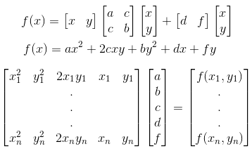 There’s no constant term in the f(x) because everything (x, y, and f) is relative to the starting position of the control point in question, so f(0) = 0, and f(x,y) is the change in the objective when moving the control point <x,y> from the initial point. There are 5 free variables, but I recommend using more than 5 new points and solving by least squares to reduce noise in the approximation. It’s also worth noting that since the (x,y) of the points are relative you can use the same ones every time and pre-compute the LDL decomposition to make solving this system of equations very fast (just do forward-backward substitution with the new f’s each time). The points I use are (1,0),(0,1),(-1,0),(0,-1),(1,1),(-1,1),(-1,-1), and (1,-1).
 Once you’ve solved for “a” to “f ” you can calculate the step-size using the same approach as Newton’s method. Because of the way the paraboloid is defined relative to the initial point we’ll always be stepping from an initial point at (0,0), and thus the gradient (g) and Hessian (H) are both taken at zero and Hd=-g is used to calculate d which is the direction we should step in to minimize this function (which is an approximation to the difference between patches connected relative to the position of a single control point). Since there are only two variables, the easiest way to solve this system of equations is with Cramer’s Rule, and that gives us the bottom explicit formula for the search direction in terms of the parabola parameters from the previous step. Once we have the direction we use our binary step-size search from the previous article to find exactly how we should move this point to reduce matching error. Iterate over all points a few times, or until they stop moving, and we’re done. Well, almost.
Homotopy
If we just made two 16×16 grids like above, laid them evenly over our images, and started optimizing it wouldn’t work. Our optimization algorithms only guarantee we’ll converge to a local minimum. We’ll go to the bottom of a valley in our error function, but if we start in the wrong valley we’ll still get the wrong answer. There is no perfect solution to the general form of this local minimum problem, but there are a few ways to combat it in special cases. The technique I use for this optical flow method is homotopy optimization.
Homotopy optimization is an optimization technique where instead of directly optimizing your true objective you start with a simpler or better conditioned objective function and as you optimize you iteratively morph the function you’re optimizing into the true objective. In our application this takes the form of a multi-scale representation (somewhat similar to image pyramids ).
We begin with just a single quadrilateral on very blurred copies of the images. We perform the optimization as above iterating over all four points and adjusting their positions on the second image to make what’s under the quads match as well as possible. Since this is only an intermediate step it is not necessary to run until complete convergence, and a small number (10-30) of iterations seems to work fine in most cases.
Once we’ve optimized a single quadrilateral we break it into 4 quadrilaterals covering the same area. We perform the optimization again on the new 9 points. Then we reduce the amount of blur (halving radius of the blur kernel seems to work well) and optimize those 9 points again. Then we split each of those 4 quads into 4 more quads and optimize the now 81 points. Reduce blur, optimize, split quads, optimize, repeat until desired level of accuracy is reached.
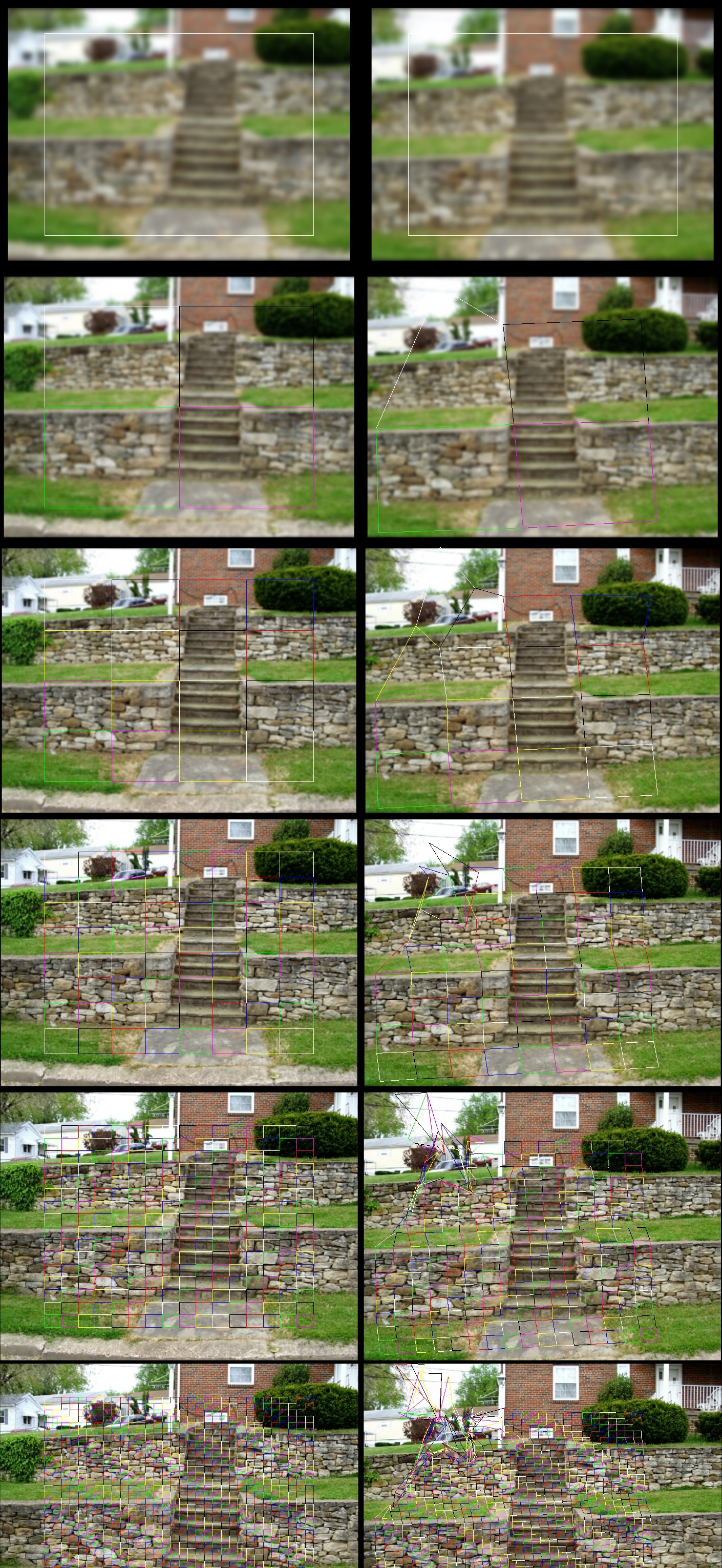
It can be a bit tricky to select the initial blur radius, the optimization iterations at each step, and the level of detail. These numbers depend heavily on the input size of the images, how close together the images were taken, and just how much detail you need for your application vs the time you’re willing to spend processing. Unfortunately, I don’t have any hard and fast rules. For the code attached to this article I scale all input images to a fixed size and use a fixed starting kernel size I found by trail and error. The number of quads quadruples at each level of detail and, roughly speaking, so does the run-time. Three to six levels of detail seems reasonable for common applications.
Conclusion
As I mentioned from the get-go this method of calculating optical flow is certainly not the fastest or the most robust to poor image conditions. It’s probably on the simple side as far as optical flow algorithms go, but It’s not the simplest possible method, which is to say you won’t find anything like it on the Wikipedia page for optical flow. It’s primary advantage over more basic techniques is a higher degree of precision covering a larger fraction of the image. These properties make it fairly well-suited to 3D reconstruction and video super resolution. It’s also worth mentioning that it’s pretty easy to detect and discard mismatches because their quads have a high matching error or because the 3D reconstruction isn’t physically possible. We’ll get into that in the next article.

When I first pitched video super resolution as a project to a professor at the University of Wisconsin-Madison I was told that it wasn’t possible to align images accurately enough to pull it off. I developed this alignment technique after 5 or 6 other attempts failed to give the desired precision. Ultimately I built a successful video super resolution system and proved that professor wrong. Unfortunately, none of the work was ever published, and since I’ve left the academic system a peer reviewed publication is unlikely.
The tag-line of this blog is “making the impossible practical”, but the articles thus far have been mostly by the book. That’s not the case for this article, and it won’t generally be the case going forward. I’m going to be mixing a lot of my own original research into the lessons, and I hope, presenting methods that are less academic and more useful for real world problems. Next up is 3D reconstruction. The code for that is already on GitHub mixed with the code for this article. Video super resolution and image hallucination are also on the queue, but I will probably hit some more optimization techniques and machine learning before I get into all of that. I hope you’ll stayed tuned, and as always let me know if you find any errors or discover any major improvements.